In this tutorial I will go through the ideas that underpin constraint programming, a technique for solving hard algorithmic problems. It is a pretty advanced technique and is an active research area, but despite this the core ideas are actually surprisingly easy to understand. After reading this tutorial hopefully you’ll understand the principles of how a constraint programming solver works.
I want this tutorial to be understandable to as many as possible, regardless of how much programming background you have. If you feel like you don’t understand it’s probably not your fault, but mine. I’ll try to make it clearer if you tell me about it (for example on the mailing list). At times the text can be a bit technical, but I try to explain things from different angles so try continue reading if you get stuck and it will hopefully be clearer.
P vs NP 🔗︎
To understand why constraint programming is desirable in the first place, let me first talk about two classes of algorithmic problems: P and NP. There are many ways to describe them using various levels of rigor. Intuitively you can think of P as the set of problems that are easy to solve, and NP as those that are probably hard to solve but easy to verify. If you give me a solution to an NP problem I can check that it is correct easily. (sidenote: Ok maybe not me, but somebody probably can. ) I say “probably” because nobody knows if they can be solved easily.
What do I mean when I say “easy” and “hard”? A slightly more precise explanation is that hard problems require search to solve and easy problems don’t. You can’t construct a solution to a hard problem, you have to do at least some trial and error.

Figure 1: Examples of time complexities. The x-axis is the input size and the y-axis execution time. Credit: Cmglee, CC BY-SA 4.0, via Wikimedia Commons
The more formal definition involves time complexity. Briefly, time complexity measures how fast the execution time grows depending on the input. In the image above you can see that \(\sqrt{n}\) and \(log_{2}(n)\) both grow very slowly. An algorithm with such a time complexity can handle large inputs without going much slower. \(2^{n}\) and \(n!\) on the other hand grow very quickly. Even for small problem sizes it can quickly become infeasible to solve because it simply takes too much time. Algorithms with time complexities \(n^{2}\), \(n \cdot log_{2}(n)\) and \(n\) are all considered to run in polynomial time.
Easy problems can be solved in polynomial time. This is the complexity class P. NP is the class of hard problems. NP does not stand for Non-Polynomial, instead it stands for Non-deterministically Polynomial. What that means is that if I have an oracle that picks a candidate solution from thin air, I can check if that candidate is a valid solution in polynomial time. What we don’t know, is whether NP problems can be solved in polynomial time or not, whether P is equal to NP or not. Nobody has given a polynomial time algorithm for an NP-problem nor have anybody proven that it is impossible. In fact, P vs NP is one of the unsolved Millenium Problems.
Constraint Programming 🔗︎
There are many problems that are in NP that we want to solve fast. For example many routing, scheduling and logistics problems lie in NP but are still important to solve quickly. These problems come in many shapes and sizes so it’s too expensive to design an optimized algorithm for each and every one of them. Instead, what we want is a general framework that can efficiently solve many classes of problems as long as a human can describe them. That way we can start solving new problems fairly quickly.
This is where Constraint Programming comes in. It is one such framework that is particularly easy to understand the internals of. So, let’s dive right into it with an example problem: n-queens.
Suppose you are given an empty \(n \times n\) chess board and \(n\) queens. The problem is to place all queens such that no queen attacks another queen. (sidenote: According to Wikipedia n-queens isn’t in NP, but it’s easy to modify it so that it is. Instead of getting an empty board, we get a board with an arbitrary amount of queens already placed. The question then becomes whether it is possible to place the remaining queens so that no queen attacks another queen. )
First approach: Pure brute force 🔗︎
Since we want to solve hard problems, and hard problems require search, let’s first start trying to solve this by a stupid brute force search, and then we can try to be smart later. Let’s create \(n^{2}\) boolean variables, one for each square. A variable should be True if a queen is placed on it and False otherwise.
First let’s just try guessing at random to get a feel for the problem.
| ♛ | |||
| ♛ | |||
| ♛ | |||
| ♛ | |||
| ♛ | ♛ | ||
The last queen we placed is attacked by two other queens, so continuing from here will only lead to an illegal solution. In fact, if we highlight all the squares that at least one queen is attacking we can see that there is only one legal square left.
| 🟥 | 🟥 | 🟥 | 🟥 |
|---|---|---|---|
| 🟥 | ♛ | 🟥 | 🟥 |
| 🟥 | 🟥 | 🟥 | ♛ |
| 🟥 | 🟥 | 🟥 |
Our random algorithm has \(1 / 13 = 8\%\) chance of guessing a valid square for our next queen, and after that we won’t have any space left to place our fourth queen. On top of all that there is no guarantee that our random algorithm won’t keep stumbling upon the same bad configurations like the one above.
Let’s try to get rid of that last problem by visiting every possible combination of queens only once. To do this we need to keep track of which combinations we have already tried, but we don’t want to store them directly as that would take too much memory. Instead we could design an algorithm that we know will go through all the possible combinations.
So, we need to do this in a systematic way. Let’s try going through the positions of the board in order, left to right and then top to bottom (the same order you would read the characters in this text), and for each position we decide if there is going to be a queen there or not. When we have placed all the queens we have we check whether this board is a solution to the problem, i.e. we check if any of the queens are attacking another queen. First let’s place the first queen in the top-left most square.
| ♛ | |||
|---|---|---|---|
Then we place the queen in the position (1, 2), (1, 3) and (1, 4).
| ♛ | ♛ | ♛ | ♛ |
|---|---|---|---|
This is obviously not a valid board so let’s undo our last move. The last move was to place the queen at (1, 4) so let’s do the opposite of that and place no queen there. Now we have a queen left to place that we set let us place it at the next available position: (2, 1), the next spot in our order.
| ♛ | ♛ | ♛ | |
|---|---|---|---|
| ♛ | |||
This is once again an invalid board, so let’s undo that.
| ♛ | ♛ | ♛ | |
|---|---|---|---|
Even if we go through and test all available places to place this queen we would always end up with an invalid board. Let us undo another move.(sidenote: You might notice that we can’t in fact put any other queens on the top row since the queen at (1, 1) will attack all of them and that we are checking a lot of board combinations unnecessarily. That is correct. Put a pin in that thought, we’ll come back to it later. )
| ♛ | ♛ | ||
|---|---|---|---|
Alright, where do we place the next queen? The answer is at (1, 4). But haven’t we already tried placing a queen there? you might ask. Yes, that is true but we haven’t placed a queen at (1, 4) while (1, 3) is empty. We are checking every single position. This might be a little hard to grasp, but it makes sense if we look at it as a tree.
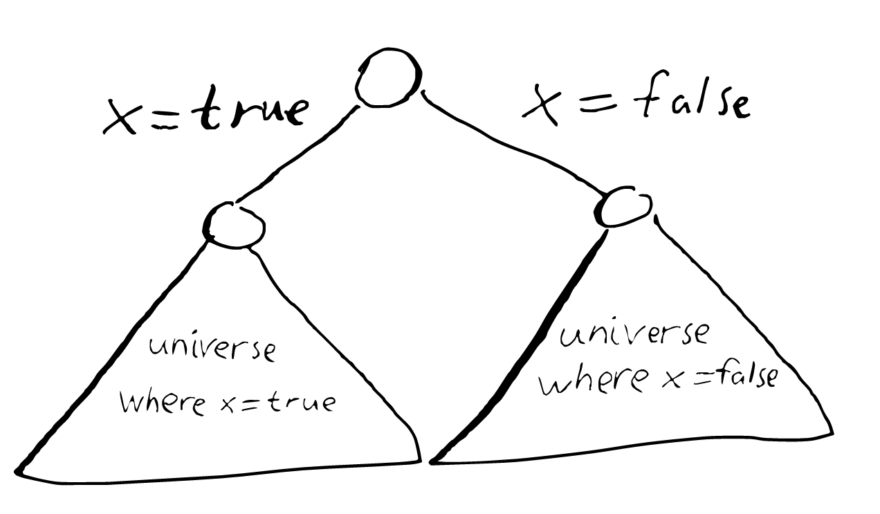
As an example, let us consider three variables X, Y and Z that can take the values true or false. We want to explore all combinations of values these three variables can take. The easiest way to do that is through recursion. Imagine you have a machine that can solve the problem, but it only works for two variables, it can give you all combinations of values for Y and Z, but not for X, Y and Z. How, then, do you use that to solve the problem? Well, X can only have two values: true and false. Let us assume that X has only one value: true. Now in this “universe” the answer to our problem is basically given by our machine. The same is true if we instead assume that X has the value false.
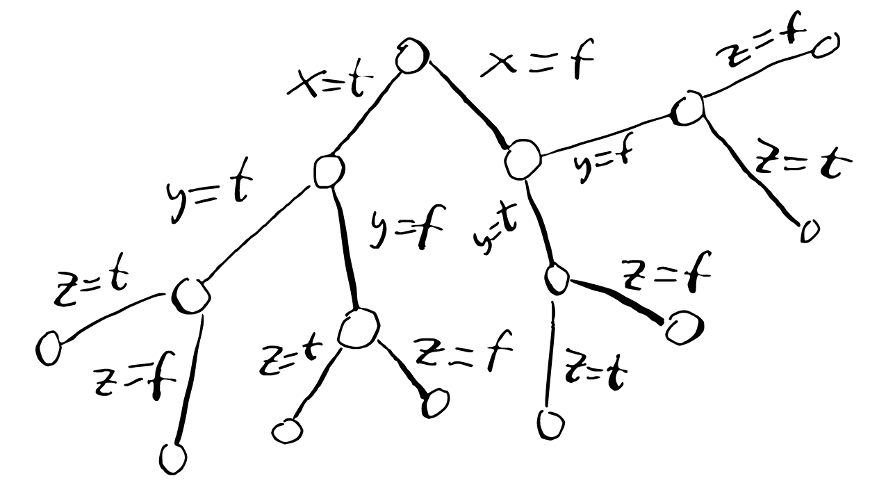
So more concretely, to explore the search space is to traverse a tree like the following one:
And the order we will traverse is the following one:
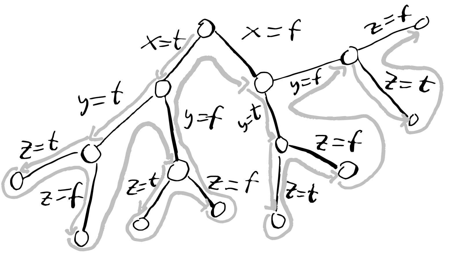
After we have explored a sub-tree, we backtrack by undoing our assumptions.
Let’s inject some intelligence 🔗︎
Observation 1 🔗︎
You might have noticed that once we have placed a queen, we can skip the rest of that row, since the queen we just placed is attacking that row and we can’t place anymore queens there. We could try implementing something off of that immediately by fiddling with some index variables but first let’s try reformulating what we know to see if we can get something easier. We know that two queens can’t be on the same row, so we know that if we place a queen we can’t place another queen on the same row. In other words we place exactly one queen per row. We have \(n\) number of queens that should be uniquely placed in \(n\) rows. That means we have \(n\) queens that each have one unknown integer value, the column coordinate. A coordinate can be represented by a number, so we can represent our queens with \(n\) numbers. By construction, using this representation no queen can attack another queen on the same row. So by just reformulating our model we got one of the queen’s attack patterns for free and shrunk the search space.
And, as a bonus, our validator has less work to do. It doesn’t need to check that queens don’t attack each other vertically as that is true now by construction.
So we shrunk the search space by realizing that we don’t need to consider placing queens on rows where we have already placed a queen. Can we do something similar for columns?
Observation 2 🔗︎
Just like with the rows, once we place a queen on a column we can’t place anymore queens in that same column, but we can’t use the same trick as before since we’ve already decided on a representation. We have to think of something new. Hmm. Once we’ve picked a column we have effectively consumed it and can’t reuse it. We could keep a set that holds the values we haven’t consumed yet. When we guess a value for a queen’s column coordinate we pick a number from that set, and remove it.
Here is an example run on a 4x4 board.
set: \(\{1, 2, 3, 4\}\)
set: \(\{2, 3, 4\}\)
| ♛ | |||
|---|---|---|---|
set: \(\{3, 4\}\)
| ♛ | |||
|---|---|---|---|
| ♛ | |||
set: \(\{4\}\)
| ♛ | |||
|---|---|---|---|
| ♛ | |||
| ♛ | |||
set: \(\{\}\)
| ♛ | |||
|---|---|---|---|
| ♛ | |||
| ♛ | |||
| ♛ |
Domains 🔗︎
Alright, now we have been able to cut down the search space significantly by intelligently deducing which values are impossible because of the queens’ vertical and horizontal movements, but what about the diagonals? At this point it’s getting a bit hard to reason about which values are still available in our search, and at least I can’t come up with a strategy to eliminate the diagonals from the search. Instead let’s back up a bit and try another approach. Instead of trying to make the search algorithm more clever let’s instead try to achieve what we want more directly. We want to keep track of which positions are still legal for a queen to have.
More generally what we want is a way to keep track of which values are still available for each variable. This is pretty close to what mathematicians call domain so let’s call it that. For now let’s keep the implementation abstract and focus on how we interact with it.
Let’s keep the idea from Observation 1. Let each queen be represented by a domain: a set of integers representing which columns she can be placed on. Each time we place a queen we know which additional squares become illegal, so we remove those squares from all the domains.
As an example, take the following 3 x 3 board with no queens placed. All domains are full.
Then when we place a queen in (1, 1) a bunch values are removed from the domains:
| ♛ | 🟥 | 🟥 |
|---|---|---|
| 🟥 | 🟥 | |
| 🟥 | 🟥 |
Backtracking 🔗︎
We can’t forget about backtracking! When we get into a dead end we still need to undo our steps. Continuing from our previous example:
| ♛ | 🟥 | 🟥 |
|---|---|---|
| 🟥 | 🟥 | |
| 🟥 | 🟥 |
Remember, we have restricted our queens to their own rows, so there is only one place we can place the queen on row 2.
| ♛ | 🟥 | 🟥 |
|---|---|---|
| 🟥 | 🟥 | ♛ |
| 🟥 | 🟥 | 🟥 |
The domain for the queens now looks like this:
| Queen | Domain |
|---|---|
| 1 | { 1 } |
| 2 | { 3 } |
| 3 | { } |
The domain of the third queen is empty, it doesn’t have any columns it can be in so we can’t get a solution this way! One or more of our guesses must have been wrong so we need to go back and try the other alternatives. But to do that we need to add back the values we removed since before the last time we made a guess. To keep it simple let’s just copy the domains each time we do a guess. When we undo a guess we restore the domains to their appropriate state from the correct copy.
We need to undo the last queen it placed, but because there was only one place to put that queen we need to undo another move. Now we’re back to the starting board.
The second option for queen one is to place it on column 2.
| 🟥 | ♛ | 🟥 |
|---|---|---|
| 🟥 | 🟥 | 🟥 |
| 🟥 |
This will of course not lead to a solution either since queen 2 doesn’t have any legal columns left.
We can also understand this backtracking from the angle of the search trees. Suppose we have this search tree with at least two integer variables X and Y with domains \({0, 1, 2}\):
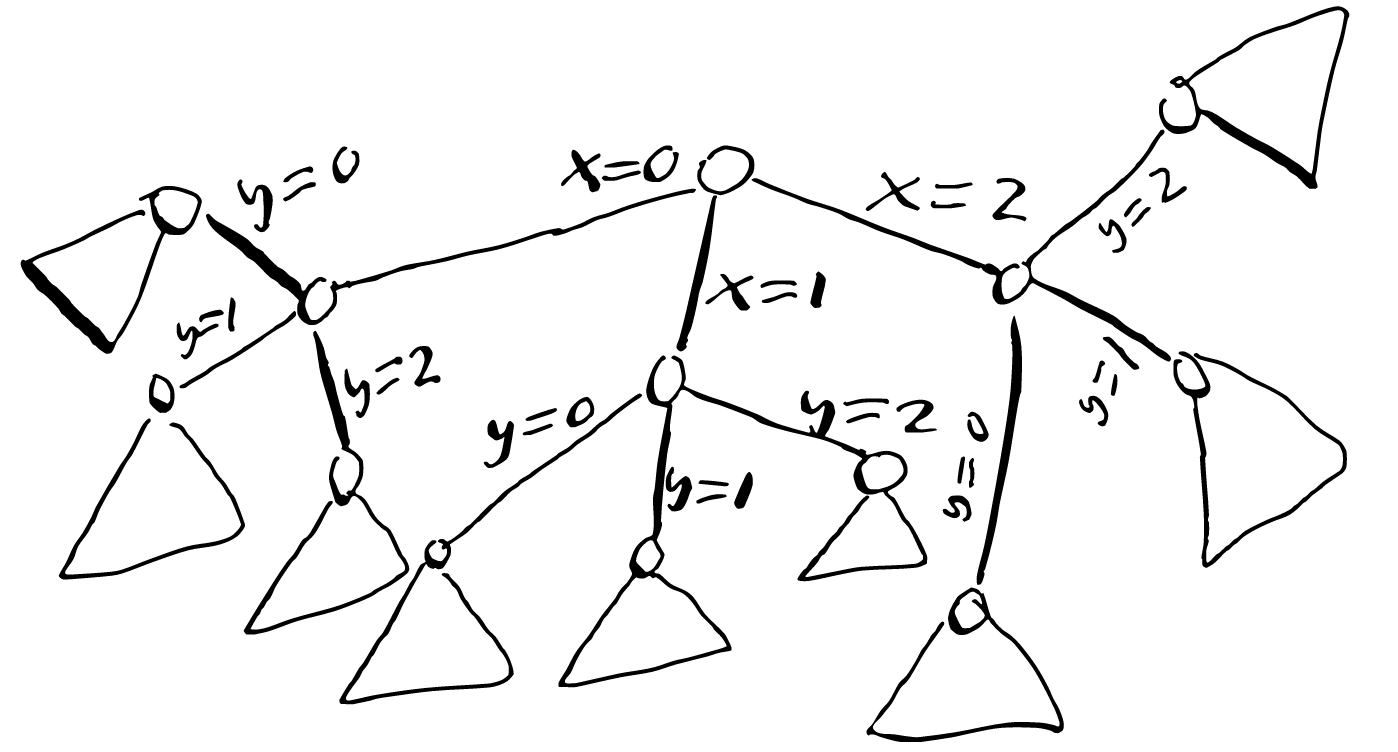
In search, each time we fix the value of X we realize somehow that the value 1 is illegal for Y, so we prune it from the Y’s domain. The resulting search tree (seen below) is much smaller. Through some (hopefully) cheap inference we could remove a potentially huge part of the search tree that would have taken a long time to traverse.
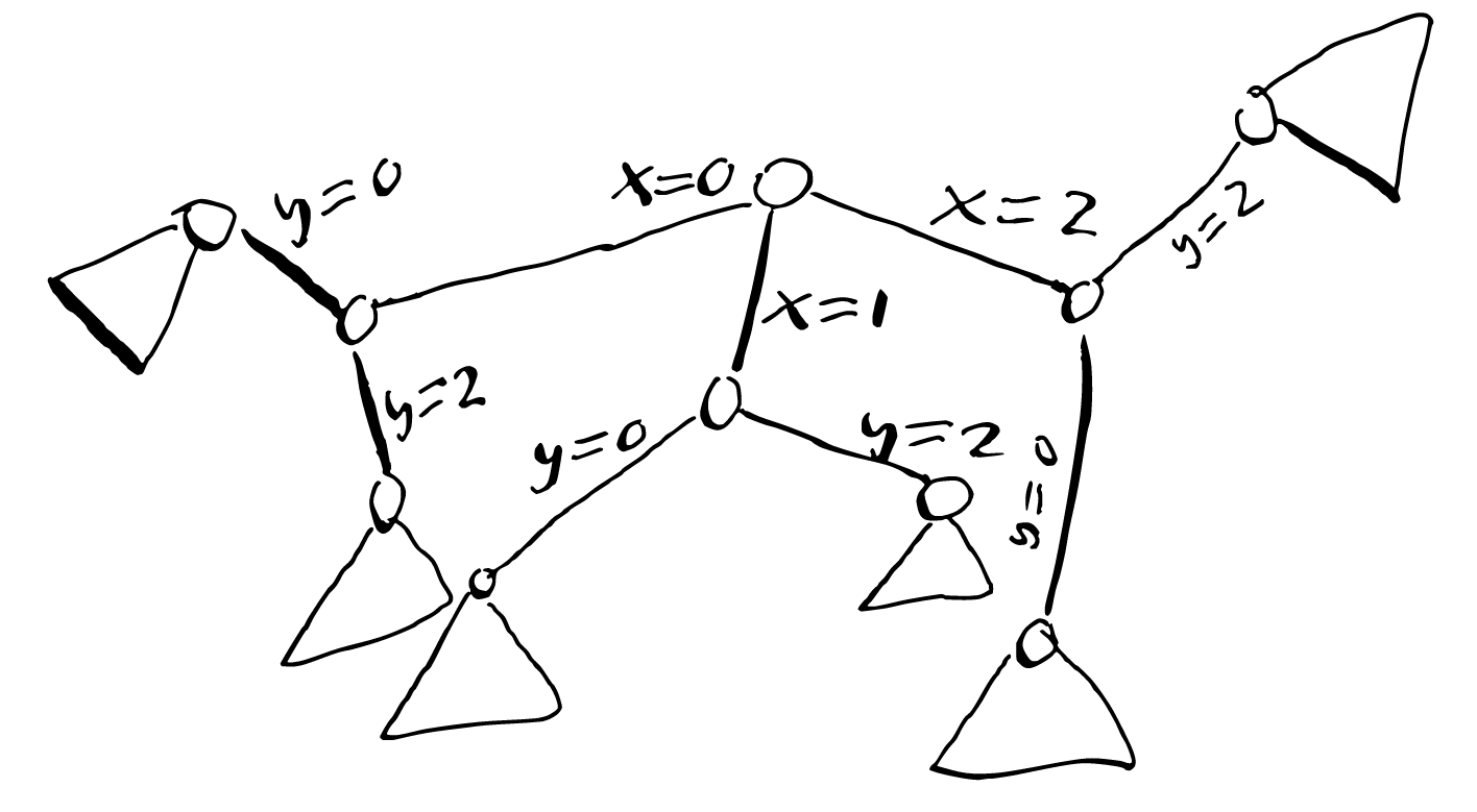
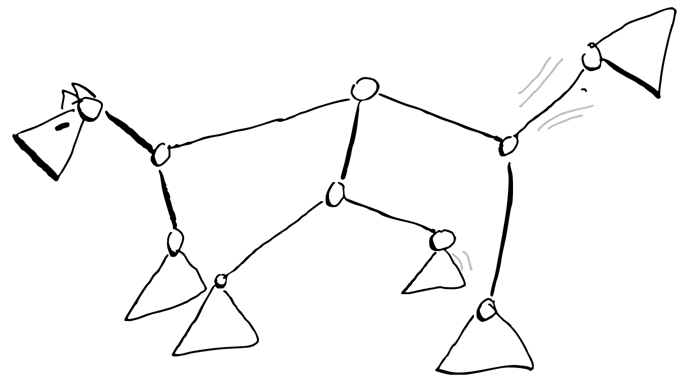
Incidentally, this search tree also looks like a dog:
More intelligence! 🔗︎
Let’s try another example to see if we can find more cases where we can be even smarter.
First let’s place queen number 1 on the first column:
| ♛ | 🟥 | 🟥 | 🟥 |
|---|---|---|---|
| 🟥 | 🟥 | ||
| 🟥 | 🟥 | ||
| 🟥 | 🟥 |
The next queen is placed on column 3, the first legal column.
| ♛ | 🟥 | 🟥 | 🟥 |
|---|---|---|---|
| 🟥 | 🟥 | ♛ | 🟥 |
| 🟥 | 🟥 | 🟥 | 🟥 |
| 🟥 | 🟥 | 🟥 |
That makes it impossible to place queen 3 so we need to backtrack.
Then let’s put the second queen on column 4:
| ♛ | 🟥 | 🟥 | 🟥 |
|---|---|---|---|
| 🟥 | 🟥 | 🟥 | ♛ |
| 🟥 | 🟥 | 🟥 | |
| 🟥 | 🟥 | 🟥 |
Hang on, queen number 3 only has one possible square to be in since all other squares in that column are crossed out. We can fill that in immediately, without any guessing!
| ♛ | 🟥 | 🟥 | 🟥 |
|---|---|---|---|
| 🟥 | 🟥 | 🟥 | ♛ |
| 🟥 | ♛ | 🟥 | 🟥 |
| 🟥 | 🟥 | 🟥 |
Alright, we just placed a queen. Even though it wasn’t through guessing we should still cross out the squares that this queen is attacking.
| ♛ | 🟥 | 🟥 | 🟥 |
|---|---|---|---|
| 🟥 | 🟥 | 🟥 | ♛ |
| 🟥 | ♛ | 🟥 | 🟥 |
| 🟥 | 🟥 | 🟥 | 🟥 |
But now there are no places to put the last queen so we have to backtrack again. It doesn’t seem to be enough to just undo the queen we placed through inference (as opposed to search) since there was only one square we could place it on. Instead we should backtrack to the last time we had to make a decision between several possibilities, the last time we did a search decision.
| ♛ | 🟥 | 🟥 | 🟥 |
|---|---|---|---|
| 🟥 | 🟥 | ||
| 🟥 | 🟥 | ||
| 🟥 | 🟥 |
However we have exhausted all possibilities for queen two here (we have tried placing it on both column 3 and 4), so we need to undo the placement of queen 1 and continue the search.
The next spot for queen 1 is column 2.
| 🟥 | ♛ | 🟥 | 🟥 |
|---|---|---|---|
| 🟥 | 🟥 | 🟥 | |
| 🟥 | 🟥 | ||
| 🟥 |
We can infer that queen 2 has to be placed at column 4.
| 🟥 | ♛ | 🟥 | 🟥 |
|---|---|---|---|
| 🟥 | 🟥 | 🟥 | ♛ |
| 🟥 | 🟥 | 🟥 | |
| 🟥 | 🟥 |
And then queen 3 can only be placed at column 1.
| 🟥 | ♛ | 🟥 | 🟥 |
|---|---|---|---|
| 🟥 | 🟥 | 🟥 | ♛ |
| ♛ | 🟥 | 🟥 | 🟥 |
| 🟥 | 🟥 | 🟥 |
And finally we deduce that queen 4 is placed at column 3, and we’ve solved the problem!
| ♛ | |||
|---|---|---|---|
| ♛ | |||
| ♛ | |||
| ♛ |
This was really fast, after two guesses we could immediately deduce that these guesses were impossible without any more guesses. And then, when we happened to guess the right placement for the first queen we got a cascading effect where inferences triggered other inferences until it solved the problem.
We should use this in our algorithm. What we noticed was that when we reduce the number of possible placements of a queen to 1 we can immediately place it, and then remove all the squares it is attacking from the other queens’ domains. This of course can shrink other queens’ domains to size 1, hopefully creating a cascade of queen placements.
Taking a step back: Generalization 🔗︎
Now that we have tasted the blood of a combinatorial puzzle we are hungry for more.(sidenote: At least I am. ) What other puzzles are similar to n-queens that we can hunt down? Sudoku feels pretty similar. We could interpret it as an n-rooks problem where each number can only attack another number of the same value, with the additional rule that a number can attack in the same 3 x 3 square. Could we solve by applying what we have learned so far?
The first thing we learned was that instead of using an \(n \times n\) array of boolean variables we could use an \(n\)-length array of integer variables with domain size \(n\). This doesn’t seem to be immediately applicable since in this case we actually need to fill in every square. So let’s use that \(n \times n\) variable array, but this time we use integer variables that signify which integer we are going to place on that square, which is basically the intuitive representation.
The second thing we learned was that we could use domains what values are still legal for each domain, and when we place a queen (or more generally fix a variable to a single value) we remove the illegal values for all other variables. The constraint that no queen is allowed to be on the same column can be reformulated as “each variable (that represents a queen’s column coordinate) has to be of different values”, or “the variables have to be all different”. That could be useful for the sudoku puzzle so let’s write that down in a more terse notation:
array [1..n] of var 1..n: q; % queen in row i is in column q[i]

constraint alldifferent(q);                       % distinct columns
The diagonal attacking patterns can also be encoded using the same constraint(sidenote: Taken from https://www.minizinc.org/doc-2.5.5/en/mzn_search.html ) (why it works isn’t important, but feel free to try to rationalize it for yourself):
constraint alldifferent([ q[i] + i | i in 1..n]); % distinct diagonals
constraint alldifferent([ q[i] - i | i in 1..n]); % upwards+downwards
Let’s see, can we use these tools to solve sudoku? We already have the representation we want, so the question is how we encode the rules of sudoku using the alldifferent constraint. Actually the rules are already basically written in terms of alldifferent:
- All squares have to have a value between 1 and 9
- The values in a single column have to be
alldifferent - The values in a single row have to be
alldifferent - The values in a single sub-square have to be
alldifferent
Using our syntax from above we can formulate it as:
array [1..9][1..9] of var 1..9: board;

% rows
constraint forall(i in 1..9) (alldifferent([board[i][j] | j in 1..9]))
% columns
constraint forall(i in 1..9) (alldifferent([board[j][i] | j in 1..9]))

% sub-squares
constraint alldifferent([board[i][j] | i in 1..3, j in 1..3])
constraint alldifferent([board[i][j] | i in 4..6, j in 1..3])
% continue for the rest of the sub-squares...
That’s all the rules we need! Since the domain of each variable is \(1..9\) and there is an alldifferent constraint on each row, column and sub-square (that all contain 9 variables) we automatically get that exactly one of each digit is present in each row, column and sub-square.
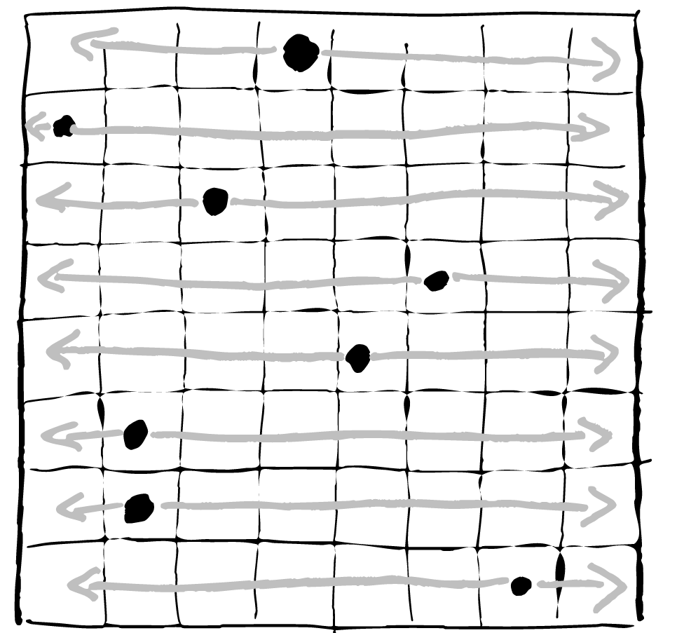
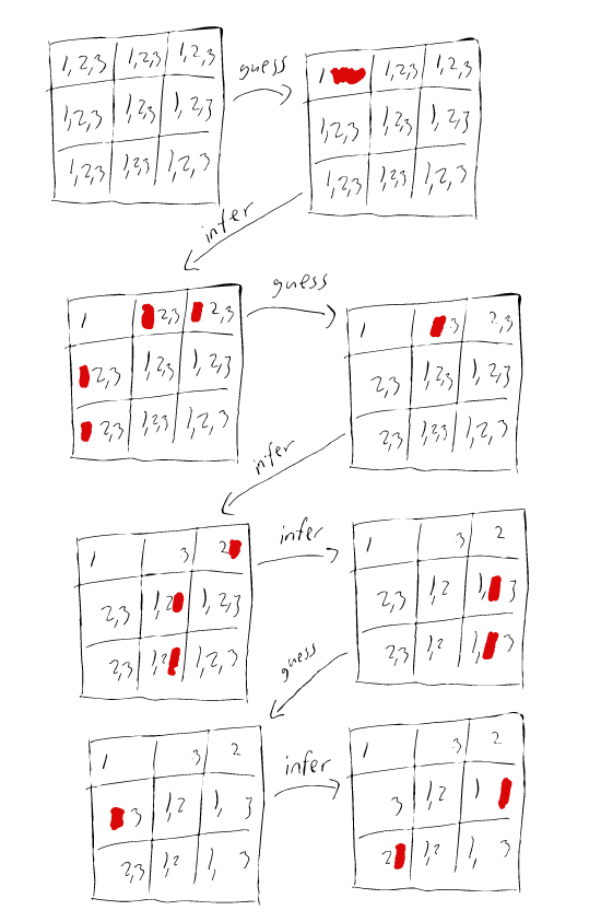
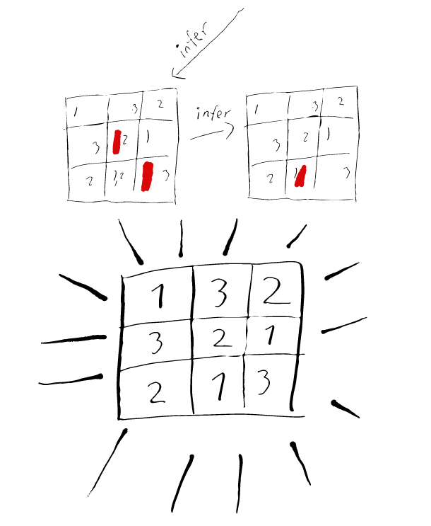
Below is an illustration of how it might look like if we used only the row and column constraint on a \(3 \times 3\) sudoku board:
Recap and generalization 🔗︎
We have a set of variables that should fulfill a set of constraints. To do that we have a data structure called a domain that keeps track of which values we haven’t ruled out yet. We have two ways to rule out values in the domain: search and inference. The search algorithm tries to exhaustively search the problem space by guessing each possible combination of values for the variables. This is slow, so to make it go faster we apply inference each time the search algorithm guesses a value for a variable. During inference, propagator algorithms remove values we know violate the constraints. When the propagator changes the state of a domain more propagators are triggered, creating a cascade of domain updates. When the propagators can’t find any more values to prune the search continues on a smaller search space. When the search needs to backtrack, we restore the state of the domains from a backup.
Notice that I didn’t specify what the constraints are. Above we exclusively used the alldifferent constraint, but there is nothing that hinders us from defining other constraints. For example we could define a constraint that says that for two variables \(x\) and \(y\), \(x > y\) must hold. To prune variables from \(x\) and \(y\) we remove all values that can’t satisfy the constraints. (sidenote: In this case we remove all \(x\) that are smaller or equal to the largest value of \(y\), and all \(y\) that are larger or equal to the smallest value of \(x\). )
Why Constraint Programming is a cool technique 🔗︎
Compared to other techniques of building solvers (e.g. Mixed Integer Programming or SAT), constraint programming is fairly high level. Users don’t have to reformulate their problem to a very specific language. Instead, high level constraints (such as alldifferent) can be implemented directly in the solver which can make the solver easier to use, and some performance can be gained since we can make optimizations that makes use of assumptions (see the different ways of implementing alldifferent for an example). The basic concepts are also easy and intuitive to understand, as this text hopefully has shown you.
Where to go next 🔗︎
There’s still so much more to learn about constraint programming. There are many more constraints to implement and optimize (for example, there is an even more efficient alldifferent implementation that uses a theorem from graph theory). In this tutorial we haven’t spent much thought on how to do search, but there are many questions there that we haven’t explored. When searching, which variable do you choose to branch on? And when you have chosen a variable, which value do you choose to fix first? How do you manage the domain’s state? When do you trigger the propagators? How hard should a propagator try when eliminating impossible values? The performance of the solver is highly dependent on the answers you choose to these questions.
If you’re curious about I highly recommend the free course for MiniCP. There you’ll be given a very bare-bones Constraint Programming solver written in Java (it’s not that bad, the flaws of Java don’t really become relevant). For the rest of the course you’ll answer the above questions when you build on that solver until it’s fairly competent.
If you want to learn more about modelling (formulating what constraints to use) there are two free courses on Coursera: Basic Modeling and Advanced Modeling.